This tutorial introduces the isorunN2O packages and provides examples of how it works and can be used. Please install isorunN2O following the instructions on GitHub, the newest version of this tutorial can always be loaded up as a vignette directly in R by calling vignette("N2O_data_reduction_tutorial") in the command line.

Loading test data

The package includes an example data set (test_run) to work with for testing and demonstration purposes. Because the original data files would be too big to include, it is stored as the cached compacted data set that the iso_save() command from the isoreader package creates from the raw data files. When you run this on your own data sets, simply change the root_folder to point to where you keep all your data (absolute path or relative to your current working directory), e.g. root_folder <- file.path("MAT", "results") and the run_folders to all the run folders you want to read in (can be one or multiple). The first time you load your own data using isoreader it may take a few minutes (speed it up using the parallel = TRUE parameter) but afterwards it will always be fast because it is already cached. The following data was read using isoreader version 1.3.0.

library(isoreader)
root_folder <- system.file("extdata", package = "isorunN2O") 
run_folders <- "test_run" # could be multiple, e.g. run_folders <- c("run1", "run2")
iso_files <- iso_read_continuous_flow(run_folders, root = root_folder) %>%
  # filter out files that have reading errors
  iso_filter_files_with_problems()

Raw data

The iso_files variable now holds all your raw data, you can look at the names of all the loaded files by running the following (here only the first 5 for brevity, also note that we’re using the %>% pipe operator to pass output from one function to the next, which might look a little strange at first but makes it more readable further on):

names(iso_files) %>% head(n=5)

## [1] "MAT25392080_P02E_run02_Conditioner-0000.dxf"
## [2] "MAT25392081_P02E_run02_N2O-0000.dxf"        
## [3] "MAT25392082_P02E_run02_N2O-0000.dxf"        
## [4] "MAT25392083_P02E_run02_N2O-0000.dxf"        
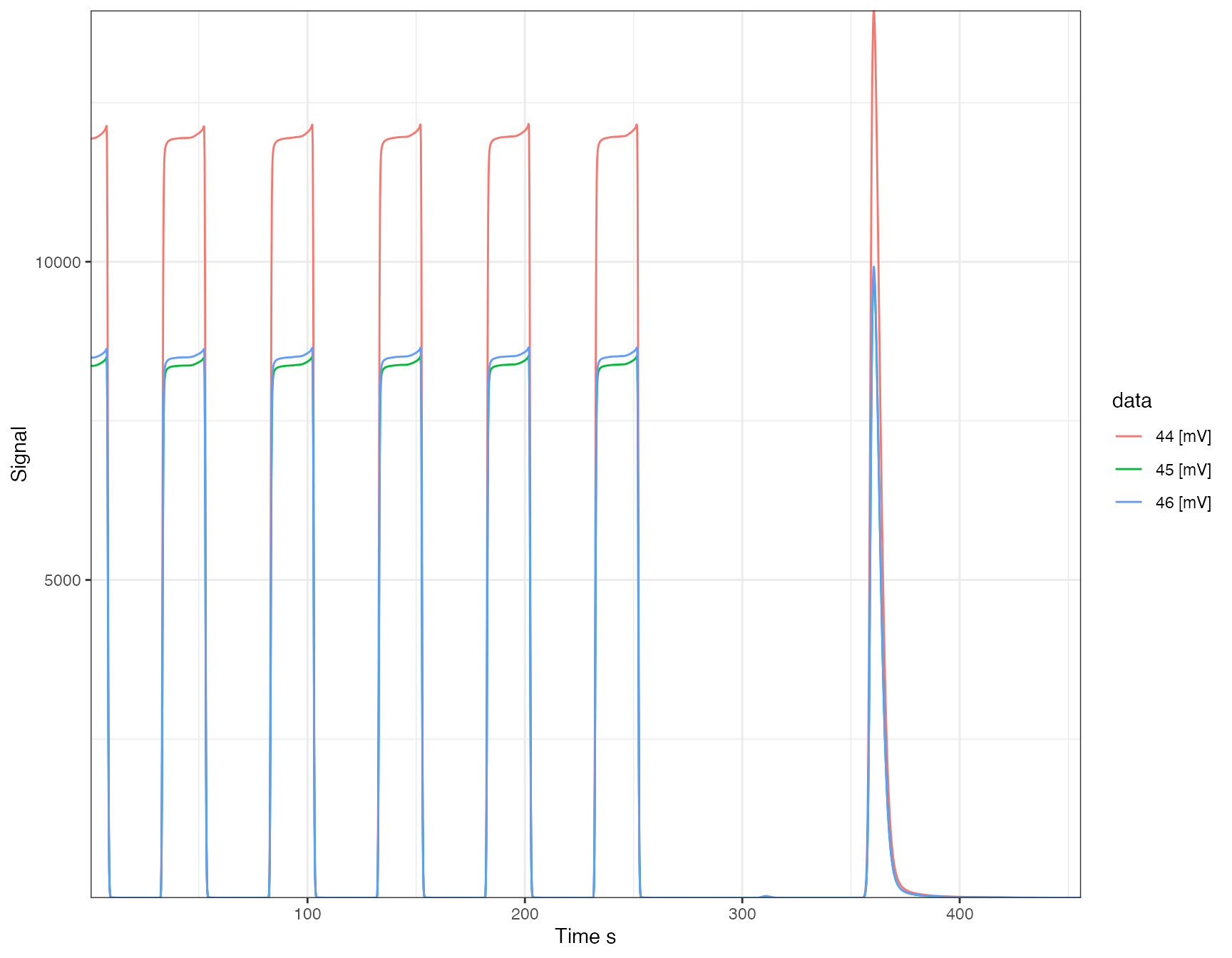
## [5] "MAT25392084_P02E_run02_N2O-0000.dxf"

You can use the file names to take a look at specific chromatograms using the functionality provided in the isoprocessor package (version 0.6.11).

library(isoprocessor)
iso_files$`MAT25392080_P02E_run02_Conditioner-0000.dxf` %>% 
  iso_plot_continuous_flow_data(color = data, panel = NULL)

Explore

If you’d like to explore the chromatograms (or really any of the data extracted from the raw data files) more, you can visually explore some of the core functionality of isoreader and isoprocessor using the isoviewer (version 0.6.11) graphical user interface with the command below (use the Close button in the GUI to return to the interactive R session):

isoviewer::iso_start_viewer()

Processing

Data processing makes use of generic data table and isotope functionality provided by the dplyr, isoreader and isoprocessor packages as well as N2O specific tools implemented in the isorunN2O package.

library(dplyr)
library(isoreader)
library(isoprocessor)
library(isorunN2O)

Data processing step 1 (first look)

In the first step, parse the file info from the sequence (take a look at what’s available with iso_get_file_info(iso_files)), pull out the peak table from the iso files (with the file info), then focus only the N2O peak (no need for the references), and focus on the main columns we are interested in. Everything is chained together with the pipe %>% operator for better readability.

df.raw <- iso_files %>%
  # extract all sample information (former parse_file_names)
  iso_mutate_file_info(
    folder = basename(dirname(file_path)),
    date = file_datetime,
    analysis = Analysis,
    run_number = parse_integer(Row),
    # category is the first part of the `Identifier 1`
    category = extract_word(`Identifier 1`, include_underscore = TRUE, include_dash = TRUE),
    # name is the full `Identifier 1` value
    name = `Identifier 1`,
    # valume information is stored in `Identifier 2`
    volume = parse_number(`Identifier 2`)
  ) %>% 
  # aggregate peak table
  iso_get_vendor_data_table(include_file_info = everything()) %>%
  # select N2O peak
  select_N2O_peak( c(360, 370)) %>% 
  # select all relevant columns 
  select_columns(folder:volume, area = `Intensity All`, d45 = `d 45N2O/44N2O`, d46 = `d 46N2O/44N2O`)

## Info: mutating file info for 181 data file(s)

## Info: aggregating vendor data table from 181 data file(s), including file info 'everything()'

## INFO: 179 N2O peaks found in 181 files (at retention time 360 - 370s), 905 other peaks discarded.

##       NOTE that no N2O peak was found in the following files (check retention time if there should be one): 
##       MAT25392086_P02E_run02_LNSW Blank-0000.dxf, MAT25392200_P02E_run02_NO SAMPLE-0000.dxf

## INFO: Selecting 10 columns (folder, date, analysis, run_number, category, name, volume, area, d45, d46), discarding 56 (file_id, file_root, file_path, file_subpath, file_datetime, file_size, Row, Peak Center, Check Ref. Dilution, H3 Stability, H3 Factor, AS Sample, AS Method, Identifier 1, Analysis, Comment, Method, measurement_info, MS_integration_time.s, Identifier 2, Nr., Start, Rt, End, Ampl 44, Ampl 45, Ampl 46, BGD 44, BGD 45, BGD 46, rIntensity 44, rIntensity 45, rIntensity 46, rIntensity All, Intensity 44, Intensity 45, Intensity 46, Intensity All, List First Peak, rR 45N2O/44N2O, rR 46N2O/44N2O, Is Ref.?, R 45N2O/44N2O, Ref. Name, rd 45N2O/44N2O, d 45N2O/44N2O, R 46N2O/44N2O, rd 46N2O/44N2O, d 46N2O/44N2O, R 18O/16O, d 18O/16O, AT% 15N/14N, R 15N/14N, d 15N/14N, AT% 18O/16O, R 17O/16O, d 17O/16O, Rps 46N2O/44N2O, Rps 45N2O/44N2O).

Now to get a sense for what the data looks like, let’s look at the first couple of rows. To look at the complete data frame, you can always call View(df.raw) or double click on the name in the Environment tab on the upper right.

df.raw %>% head(n=5)

## # A tibble: 5 x 10
##   folder date                analysis run_number category name  volume     area
##   <chr>  <dttm>              <chr>         <int> <chr>    <chr>  <dbl> <dbl[Vs>
## 1 test_… 2015-03-03 10:55:03 MAT2539…          1 Conditi… Cond…     NA 80.65752
## 2 test_… 2015-03-03 11:04:42 MAT2539…          2 N2O      N2O       20 82.40901
## 3 test_… 2015-03-03 11:14:20 MAT2539…          3 N2O      N2O       20 81.97664
## 4 test_… 2015-03-03 11:23:58 MAT2539…          4 N2O      N2O       20 82.40488
## 5 test_… 2015-03-03 11:33:36 MAT2539…          5 N2O      N2O       20 81.98561
## # … with 2 more variables: d45 <dbl[permil]>, d46 <dbl[permil]>

To check the category makeup of your run, make use of some handy dplyr functionality:

df.raw %>% group_by(category) %>% tally()

## # A tibble: 7 x 2
##   category        n
##   <chr>       <int>
## 1 Background      1
## 2 Conditioner     1
## 3 DPR             5
## 4 IAEA-NO3       28
## 5 N2O            22
## 6 P02E           94
## 7 USGS-34        28

Additionally, isoprocessor provides convenience functions for inspecting the data including iso_summarize_data_table(). Formatting options for data tables are provided by the function kable from the knitr package, which we’ll use here to get column style output.

df.raw %>% group_by(category) %>% 
  # summarize area, d45 and d46 for each category
  iso_summarize_data_table(area, d45, d46) %>%
  # format for easier display
  knitr::kable()

category	n	area mean	area sd	d45 mean	d45 sd	d46 mean	d46 sd
Background	1	0.2560503	NA	12.2815112	NA	-2.0765722	NA
Conditioner	1	80.6575200	NA	0.6003229	NA	-0.8004934	NA
DPR	5	90.3956770	1.378090	5.3718510	0.0489823	-3.0800053	0.1901865
IAEA-NO3	28	86.3229634	1.234719	5.3311431	0.1064835	19.1541208	0.2589260
N2O	22	81.8241760	1.899788	0.6362417	0.0679540	-0.8060828	0.1094067
P02E	94	87.1925131	1.143907	6.1176044	0.5982852	-2.7215962	0.5012561
USGS-34	28	86.4001330	1.257426	-2.1204132	0.0481770	-31.8621068	0.1768753

To further hone in on different data groups, simply modify the group_by:

df.raw %>% group_by(category, name) %>% 
  iso_summarize_data_table(area, d45, d46, cutoff = 3)%>% 
  knitr::kable()

category	name	n	area mean	area sd	d45 mean	d45 sd	d46 mean	d46 sd
DPR	DPR	5	90.39568	1.3780903	5.3718510	0.0489823	-3.0800053	0.1901865
IAEA-NO3	IAEA-NO3 35uM	13	86.87103	0.9617826	5.3319129	0.1445695	19.1446368	0.3419803
IAEA-NO3	IAEA-NO3 45uM	13	86.02042	0.9624278	5.3435809	0.0535936	19.1994459	0.1441963
N2O	N2O	22	81.82418	1.8997884	0.6362417	0.0679540	-0.8060828	0.1094067
USGS-34	USGS-34 35uM	13	87.01429	1.1653868	-2.1001361	0.0383784	-31.7350374	0.0802141
USGS-34	USGS-34 45uM	13	85.66835	1.0505273	-2.1292964	0.0480026	-31.9908451	0.1685208

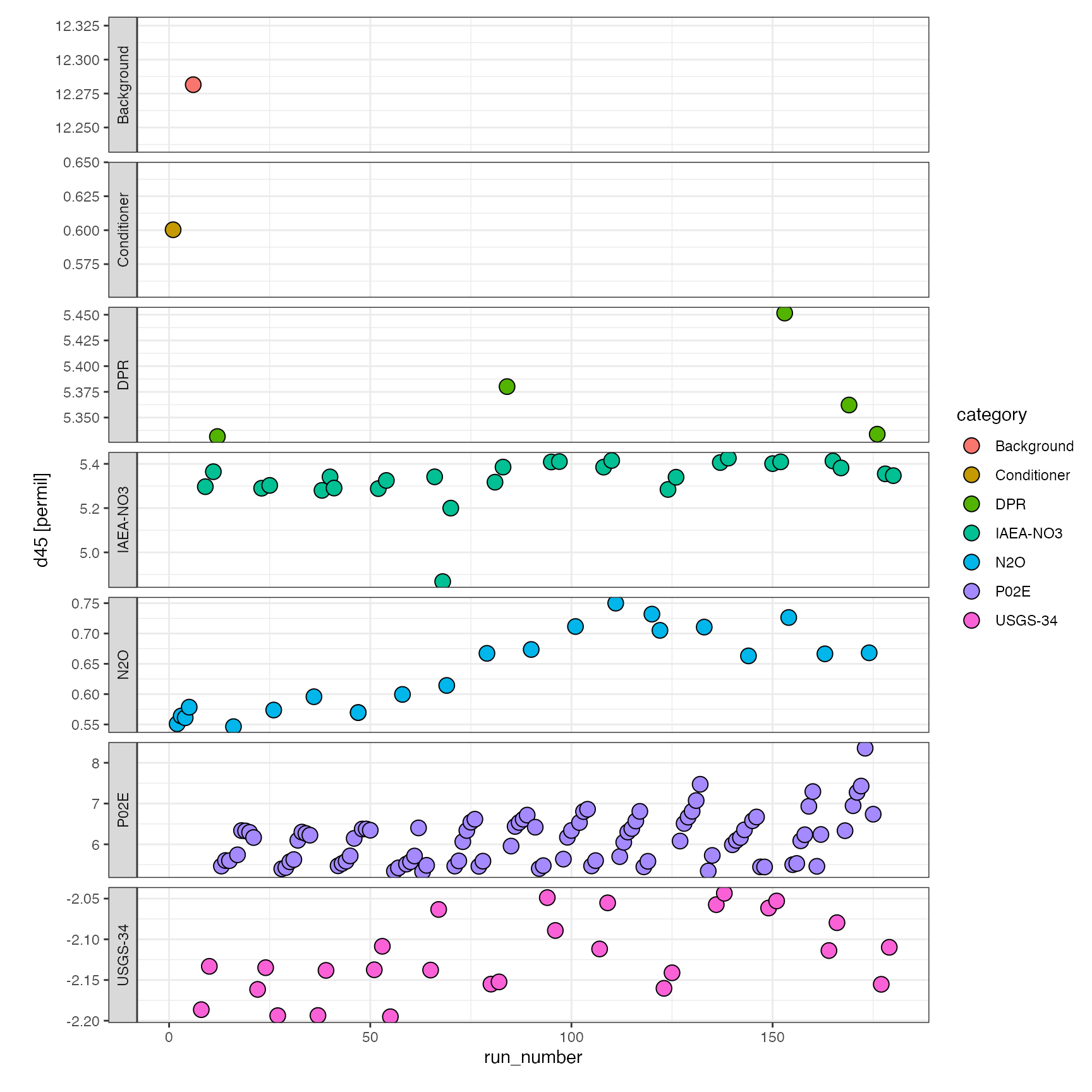
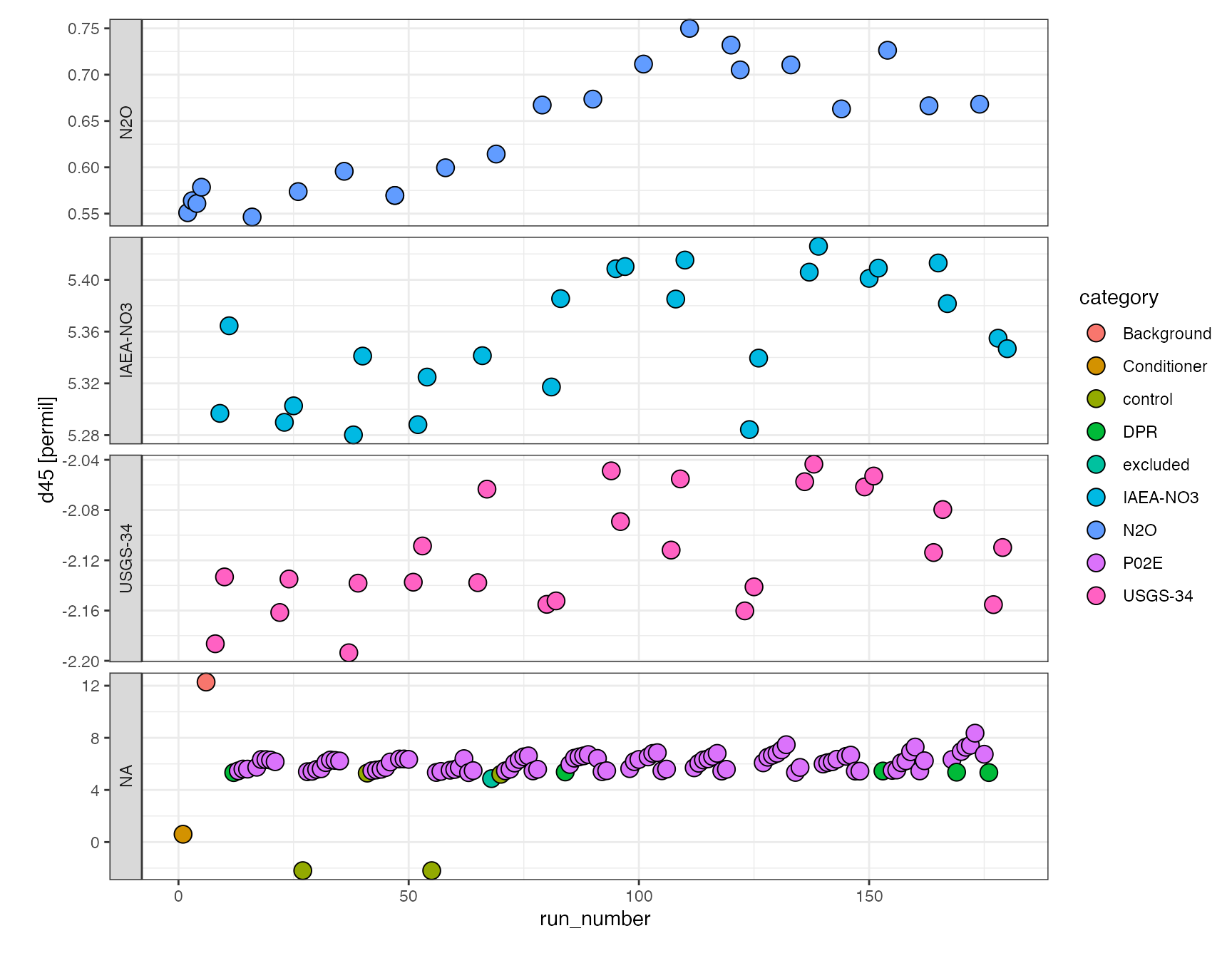
For a visual first look at the data, you can use versatile ?iso_plot_data function, which generates a ggplot:

library(ggplot2)
df.raw %>% iso_plot_data(
  x = run_number, y = d45, points = TRUE,
  # shape = 21 with fill makes data points with black borders
  shape = 21, fill = category, 
  panel = category ~ .
)

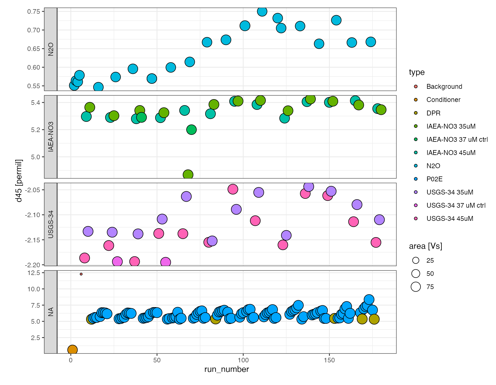
or a little bit more elaborate specifying in more detail how to color/fill and panel the overview plot:

df.raw %>% iso_plot_data(
  x = run_number, y = d45, points = TRUE,
  size = area,
  shape = 21, fill = c(type = ifelse(category %in% c("IAEA-NO3", "USGS-34"), name, category)), 
  panel = factor(category, levels = c("N2O", "IAEA-NO3", "USGS-34")) ~ .
)

or as an interactive plot (mouse-over information and zooming), which is a little easier for data exploration (make_interactive() makes the last plot interactive by default):

library(plotly)
ggplotly(dynamicTicks = TRUE)

Data processing step 2 (continued)

From the first look it is clear that there are couple of things we need to consider, there is one sample that was marked as questionable during injection (#68) which we’d like to exclude for now, there were also a couple of samples that were controls rather than standards and should go into their own category. Lastly, it appears there is some drift so we will want to evaluate that.

Drift correction

The evaluate_drift function provides a number of different strategies for evaluating drift using different correction methods, here we’re trying a polynomial fit (method = "loess") and are correcting with the standards as well as N2O. We also want to see a summary plot of the drift using plot = TRUE (the default), which will plot the drift polynomials on top of the original data (normalized to average isotope values in each group) and the residuals after applying the correction. For details look at the ?evaluate_drift help. The drift correction stores the drift corrected values in d45.drift and d46.drift.

df.drift <- df.cat %>% 
  evaluate_drift(
    d45, d46, correct = TRUE, plot = TRUE,
    correct_with = category %in% c("USGS-34", "IAEA-NO3", "N2O"),
    method = "loess"
  )

## INFO: 179 N2O analyses drift corrected (new data columns 'd45.drift' & 'd46.drift', and parameter 'p.drift' added) 
##       Used the 'loess' method with included categories 'N2O, USGS-34, IAEA-NO3'. 
##       Residual sum of squares: 0.282 (d45), 0.722 (d46) 
##       Standard deviations in d45/d46 before and after drift correction, by groupings: 
##       Before: 0.04/0.14 (IAEA-NO3 35uM), 0.05/0.14 (IAEA-NO3 45uM), 0.07/0.11 (N2O), 0.04/0.08 (USGS-34 35uM), 0.05/0.17 (USGS-34 45uM) 
##       After: 0.03/0.11 (IAEA-NO3 35uM), 0.04/0.11 (IAEA-NO3 45uM), 0.03/0.03 (N2O), 0.04/0.07 (USGS-34 35uM), 0.03/0.12 (USGS-34 45uM)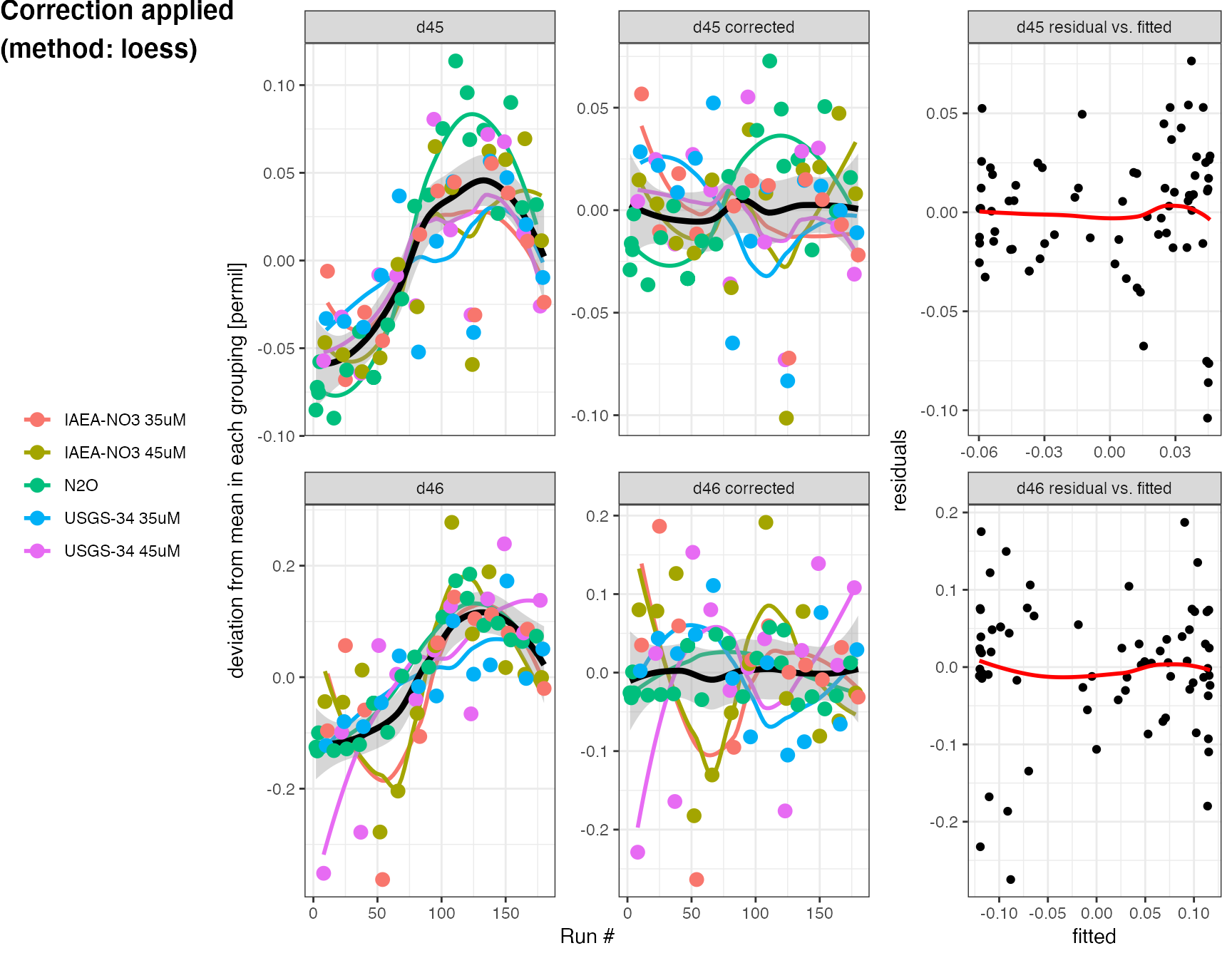

Let’s take a quick look how we’re doing after drift correction:

df.drift %>% 
  iso_plot_data(
    x = run_number, y = d45, points = TRUE,
    shape = 21, fill = category,
    panel = factor(category, levels = c("N2O", "IAEA-NO3", "USGS-34")) ~ .
  )

Data processing step 3 (continued)

Now that we’re drift corrected, time to switch to \(\delta^{15}N\) and \(\delta^{18}O\) space and calibrate against our standards.

O17 correction

We’re doing the O17 correction here (instead of before the drift) but it is a matter of discussion whether drift correction or O17 correction should be applied first. The O17 correction introduces new columns d15.raw and d18.raw.

df.O17 <- df.drift %>%
  correct_N2O_for_17O(d45.drift, d46.drift) %>% 
  # no longer need these columns now that we're in d15 and d18 space
  select_columns(-d45, -d45.drift, -d46, -d46.drift)

## INFO: 179 N2O analyses were corrected for 17O (new columns 'd15.raw' and 'd18.raw', and parameter 'p.17Ocor' added). 
##       Correction effects: mean d45 = 4.013 with resulting d15 = 4.322, mean d46 = -3.619 with resulting d18 = -3.711 [permil] 
##       Correction term constants: k46 = 1.0081, k45 = -0.0157, k17 = -0.0006, k45x45 = -0.0075, k45x17 = -0.0007, k17x17 = 0.0001

## INFO: Selecting 12 columns (folder, date, analysis, run_number, category, name, volume, area, p.drift, p.17Ocor, d15.raw, d18.raw), discarding 4 (d45, d46, d45.drift, d46.drift).

Calibration

Last steps are calculating the background (see ?calculate_background), calculating concentrations (see ?calculate_concentrations) and then calibrating \(\delta^{15}N\) and \(\delta^{18}O\) (see ?calibrate_d15 and ?calibrate_d18). Note that the background calculation is not currently used for calibration since only multi-point calibration is implemented but it’s a good check to see its value.

df.cal <- df.O17 %>% 
  calculate_background(area) %>%
  calculate_concentrations(area, volume, conc_pattern = "(\\d+)uM", 
                           standards = category %in% c("USGS-34", "IAEA-NO3")) %>% 
  calibrate_d15(d15.raw, standards = c(`USGS-34` = -1.8, `IAEA-NO3` = 4.7)) %>%
  calibrate_d18(d18.raw, cell_volume = 1.5, standards = c(`USGS-34` = -27.93, `IAEA-NO3` = 25.61))

## INFO: the category of 1 analyses was changed to 'background' (by applying criteria 'name %in% c("background", "Background")')

## INFO: bacterial background identified and area stored in parameter column 'p.bgrd': 0.256

## INFO: NOx concentrations and injection amounts (new columns 'conc' and 'amount') calculated from 35uM (25x) & 45uM (26x) standards 
##       Parameter columns mass spec signal 'p.yield' (4.346) and effective 'p.run_size' (19.87) added.

## INFO: d15 values calibrated (new columm 'd15.cal') using USGS-34 (-1.8) & IAEA-NO3 (4.7) --> stored in 'p.d15_stds' 
##       Regression: -0.4+-0.1 (d15/A, p=0.01), NA (1/A, p=NA), 0.434+-0.006 (intercept, p=3e-52)
##       Inferred reference gas isotopic composition: -0.434+-0.006 permil (added as 'p.ref_gas_d15')
##       Inferred bacterial background area: 0.4+-0.1 (added as 'p.bgrd_area') & isotopic composition: NA permil (added as 'p.bgrd_d15')

## INFO: d18 values calibrated (new columm 'd18.cal') using USGS-34 (-27.93) & IAEA-NO3 (25.61) --> stored in 'p.d18_stds' 
##       Effective concentration dependence of calibration regression taken into account. 
##       Parameter columns for calibration (measured vs. true * concentration): 
##       'p.d18_m_true' (0.897), 'p.d18_m_conc' (-0.195), 'p.d18_m_true:conc' (0.006) and intercept 'p.d18_b' (-3.359) added.

Summary

At the end of the data processing, there are a couple of ways to summarize the data, including the iso_summmarize_data_table() introduced earlier (here used to compare the raw vs. calibrated values with different groupings), but also generate_parameter_table, which summarizes all the parameters recorded from the data processing calls:

df.cal %>% group_by(category) %>% 
  iso_summarize_data_table(cutoff = 3, d15.raw, d15.cal, d18.raw, d18.cal) %>% 
  arrange(desc(n)) %>%
  knitr::kable()

category	n	d15.cal mean	d15.cal sd	d15.raw mean	d15.raw sd	d18.cal mean	d18.cal sd	d18.raw mean	d18.raw sd
P02E	94	6.0956732	0.6094777	6.5042718	0.6069220	2.587674	0.5118533	-2.8477645	0.4780328
USGS-34	26	-1.8000000	0.0379842	-1.3582935	0.0378249	-27.930000	0.1304666	-32.0829099	0.1622549
IAEA-NO3	25	4.7000000	0.0380504	5.1144509	0.0378909	25.610000	0.1095895	19.2734467	0.1056631
N2O	22	0.2647725	0.0318884	0.6978211	0.0317547	3.016624	0.0387814	-0.8080363	0.0348689
DPR	5	5.3180632	0.0352613	5.7299224	0.0351135	2.246454	0.1796061	-3.2040916	0.1761414
control	4	1.3876690	3.7297571	1.8160091	3.7141176	-1.227081	30.7282743	-6.4466047	29.4645749

df.cal %>% 
  generate_parameter_table() %>% 
  knitr::kable()

p.drift	p.17Ocor	p.bgrd	p.run_size	p.yield	p.d15_stds	p.ref_gas_d15	p.ref_gas_d15.err	p.bgrd_area	p.bgrd_area.err	p.bgrd_d15	p.bgrd_d15.err	p.d18_stds	p.d18_m_true	p.d18_m_conc	p.d18_m_true:conc	p.d18_b
loess (span: 0.75): N2O, USGS-34, IAEA-NO3	scaling=0.52; ref 17R=0.0003799, 18R=0.0020052, 15N=0.0036782	0.2560503	19.87353	4.345999	USGS-34 (-1.8) & IAEA-NO3 (4.7)	-0.4341588	0.0057633	0.362169	0.140907	NA	NA	USGS-34 (-27.93) & IAEA-NO3 (25.61)	0.896706	-0.1948884	0.0063048	-3.359054

And of course visually, e.g. in an interactive plot with additional mouseover info using the label parameter and iso_format function:

df.cal %>% 
  iso_plot_data(
    x = run_number, y = d15.cal, points = TRUE,
    size = amount,
    shape = 21, fill = c(type = ifelse(category %in% c("IAEA-NO3", "USGS-34"), name, category)),
    panel = factor(category, levels = c("N2O", "IAEA-NO3", "USGS-34")) ~ .,
    label = c(info = iso_format(
      NULL = name,
      d15 = round(d15.cal, 2),
      d18 = round(d18.cal, 2),
      amount = round(amount, 3)
    ))
  ) %>%
  ggplotly(dynamicTicks = TRUE, tooltip = c("fill", "label"))

And some simpler single data plots (using filter from the dplyr pakcage) to look specifically at the samples and DPR control.

df.cal %>% 
  filter(category %in% c("P02E", "DPR")) %>% 
  iso_plot_data(
    x = run_number, y = c(d15.cal, d18.cal), points = TRUE,
    shape = 21, fill = c(info = paste(category, panel))
  ) %>% 
  ggplotly(dynamicTicks = TRUE)

Additional customization is also possible using ggplot functionality, for example can use the shape parameter for symbol differentiation, and to visualize all the standards’ key values in separate panels, can make use of facet_wrap:

plot <-
  df.cal %>% 
  filter(category %in% c("IAEA-NO3", "USGS-34")) %>%
  iso_plot_data(
    x = run_number, y = c(amount, d15.cal, d18.cal), points = TRUE,
    shape = name, fill = name, # use multiple shapes, define with scale_shape_manual
    label = c(info = iso_format(
      `#` = run_number,
      d15 = round(d15.cal, 2),
      d18 = round(d18.cal, 2)
    ))
  ) +
  facet_wrap(panel ~ category, scales = "free", ncol = 2) +
  scale_shape_manual(values = 21:25)

ggplotly(p = plot, dynamicTicks = TRUE, tooltip = c("fill", "label"))

Export data

At any point during the process, if you like to export data as excel, this is easy with iso_export_data_to_excel (here using a couple of filter options in select to skip parameters and raw values, and using arrange to sort the data):

df.cal %>% 
  select(-starts_with("p."), -ends_with(".raw"), -ends_with(".drift"), d15 = d15.cal, d18 = d18.cal) %>%
  arrange(category, name) %>%
  iso_export_data_to_excel(filepath = "export.xlsx")

## Info: exporting datasets 'Sheet1' into Excel file 'export.xlsx'... finished.

N2O data reduction tutorial

Sebastian Kopf

2021-04-13